Painting with Random Walks

Figure 1. Random walk in dimension four. 38,000 moves

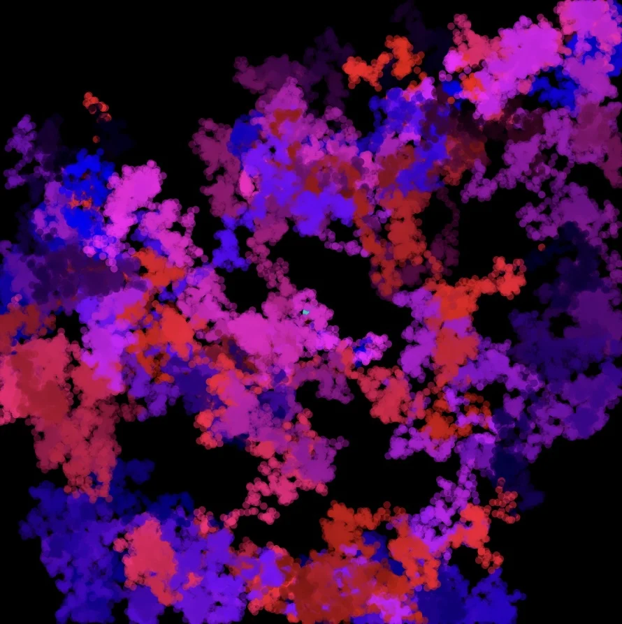
The image on the left is the result of a process called random walk. We are going to describe how to make such pictures, but to do so we must begin at the beginning, with the simplest version of this process.

Imagine a man, we will call him Joe, who has been commanded to dance along a staight line. He begins at position \(x = 0\). At each beat of the drum, he takes a step one unit to the right or one unit to the left. How does he decide in which direction to move? The rules of the dance require him to flip a coin. If it comes up heads, he moves one unit to right. If it comes up tails, he moves to the right. It is a bizarre, jerky dance, performed as if Joe were drunk.

Below is an example of one of Joe’s random walks. The 116th number is -1, so at that point Joe dies: he is out of bounds.

10,11,12,13,12,13,12,13,14,15,14,13,12,11,10,
11,12,11,10,9,10,11,10,9,10,9,10,9,10,9,8,9,
10,9,10,11,12,11,10,11,12,13,14,13,12,11,10,
9,8,7,6,7,6,7,6,5,4,3,4,3,4,5,4,5,6,7,8,7,8,
9,10,9,8,7,8,9,8,9,8,9,10,9,10,9,10,9,8,7,6,
5,4,5,4,5,6,7,6,5,6,5,4,3,2,1,0,1,2,3,2,3,4,x```
3,2,1,0,-1

Here is a less macabre version of the same random walk. This time Joe visits a casino where he can play “coin toss.” He begins by putting 10 1-dollar chips on the table. The manager of the game, lets call him Mario, flips a coin. If it comes up heads, the Mario gives Joe a 1-dollar chip. If it comes up tails, Mario takes one of Joe’s chips. In the game above, Joe keeps playing until he loses all his money. If you study the game, you see that at one point he has increased is initial capital by 50%, after which he goes loses money, never to reach that 50% gain again.

There is much more to be said about this simple gambling model, but lets’ forge on to see how to make “paintings” like Figure 1. Such a painting is a series of colored dots. To specify a dot, we must specify both position and color. Position is given by a pair of numbers \((x,y)\) as we learned in analytic geometry class in calculus. Color in our case is gotten by mixing red light with blue light. Since this is what computers like, we specify the red value by an integer \(r\) in the range \(0 \le r \le 255\), and the same with the blue value \(b\). Thus color is also specified by a pair of numbers \((r,b)\). By analogy, we think of \((r,b)\) as a point in a 2-dimensional color space, just as \((x,y)\) is a point in a 2-dimensional physical space. Now what about the colored dots? Well, they are specified by both position and color, and so by a 4-tuple \((x,y,r,b)\). Again by a analogy, this is a point is a 4-dimensional space, the space of colored dots.

One way to draw an image using colored dots is to start with an initial dot, say \(d_0 = (0,0,255,0)\). This is a red dot at the origin. Now we make repeated random changes to \(x, y, r\) and \(b\), generating a sequence of dots \(d_0, d_1, d_2, \ldots\). This is our picture!

There is more to be said, because for one thing our picture takes up a square in the plane and as the random walker moves about, he will wander beyond the boundary of the square. How should we handle that? Also the \(r\) and \(b\) values are supposed to satisfy the inequalities \(0 \le r, b \le 255\). Eventually they get too small or too large. What do we do? This is a story for another day.

You can run the random walk simulation here. And here is the source code. The app is writen in Elm